神经网络的学习 ¶

约 1816 个字 277 行代码预计阅读时间 11 分钟

简介 ¶

传统机器学习提取特征量，再用机器学习技术学习这些特征量的模式。

神经网络直接学习图像本身。

深度学习有时也称为端到端机器学习（end-to-end machine learning）。

损失函数 ¶

损失函数是表示神经网络性能的“恶劣程度”的指标，即当前的神经网络对监督数据在多大程度上不拟合，在多大程度上不一致。

均方误差（mean squared error）¶

均方误差是神经网络中常用的损失函数，定义如下：

\[ E=\frac{1}{2}\displaystyle\sum_k(y_k-t_k)^2 \]

\(y_k\) 是表示神经网络的输出，\(t_k\) 表示监督数据，\(k\) 表示数据的维数。

import numpy as np


def mean_squared_error(y, t):
    return 0.5 * np.sum((y - t) ** 2)


y = [0.1, 0.05, 0.6, 0.0, 0.05, 0.1, 0.0, 0.1, 0.0, 0.0]
t = [0, 0, 1, 0, 0, 0, 0, 0, 0, 0]

mse = mean_squared_error(np.array(y), np.array(t))
print(mse)
# 0.09750000000000003

one-hot 表示

将正确解标签表示为 1，其他标签表示为 0 的表示方法称为 one-hot 表示，即是独热编码。

交叉熵误差（cross entropy error）¶

交叉熵误差是神经网络中常用的损失函数，定义如下：

\[ E=-\displaystyle\sum_kt_k\log{y_k} \]

\(y_k\) 是表示神经网络的输出，\(t_k\) 表示监督数据，\(k\) 表示数据的维数，log 表示以 e 为底的自然对数 ln。

因为 \(t_k\) 采用 one-hot 表示方式，其中只有正确解标签的索引为 1，所以实际上只计算对应正确解标签的输出的自然对数，那么此时交叉熵误差的值是由正确解标签所对应的输出结果决定的。

正确解标签对应的输出越大，误差的值越接近 0；当输出为 1 时，交叉熵误差为 0。

def cross_entropy_error(y, t):
    delta = 1e-7  # 防止log(0)情况
    return -np.sum(t * np.log(y + delta))

t = [0, 0, 1, 0, 0, 0, 0, 0, 0, 0]
y = [0.1, 0.05, 0.6, 0.0, 0.05, 0.1, 0.0, 0.1, 0.0, 0.0]

cross_entropy_error(np.array(y), np.array(t))
#0.510825457099338

为了防止出现log(0)=-Inf的情况导致无法运算，所以加了一个微小值delta。

mini-batch 学习 ¶

前面介绍的损失函数的例子中考虑的都是针对单个数据的损失函数，如果要求所有训练数据的损失函数的总和，以交叉熵误差为例：

\[ E=-\frac{1}{N}\displaystyle{\sum_n\sum_kt_{nk}\log{y_{nk}}} \]

\(N\) 表示训练数据的总数，\(n\) 表示训练数据的索引，\(k\) 表示数据的维数，\(y_{nk}\) 表示神经网络对第 n 个训练数据的第 k 个输出，\(t_{nk}\) 表示第 n 个训练数据的监督数据。

除以 n 的目的

除以 N 进行正规化。通过除以N，可以求单个数据的“平均损失函数”。通过这样的平均化，可以获得和训练数据的数量无关的统一指标。

定义 ¶

定义 : 我们从全部数据中选出一部分，作为全部数据的“近似”。神经网络的学习也是从训练数据中选出一批数据（称为 mini-batch, 小批量），然后对每个 mini-batch 进行学习。这种学习方式称为 mini-batch 学习。

import sys, os
sys.path.append(os.pardir)
import numpy as np
from dataset.mnist import load_mnist

(x_train, t_train), (x_test, t_test) = load_mnist(normalize=True, one_hot_label=True)

print(x_train.shape)# (60000, 784)
print(t_train.shape)# (60000, 10)

读入 MNIST 的数据之后，选取小批量

train_size = x_train.shape[0]
batch_size = 10
batch_mask = np.random.choice(train_size, batch_size)
x_batch = x_train[batch_mask]
t_batch = t_train[batch_mask]

交叉熵误差 ¶

\[ E=-\displaystyle\sum_kt_k\log{y_k} \]

mini-batch 误差 ¶

可以理解为从大样本中抽取的小批量数据，代表总体进行计算

我们来实现一个可以同时处理单个数据和批量数据（数据作为 batch 集中输入）两种情况的函数。

def cross_entropy_error(y,t):
    delta = 1e-7
    if y.ndim == 1:
        y = y.reshape(1, y.size)
        t = t.reshape(1, t.size)
    
    batch_size = y.shape[0]
    return -np.sum(t * np.log(y + delta)) / batch_size

为什么有一个 delta

函数内部在计算 np.log 时，加上了一个微小值 delta。这是因为，当出现 np.log(0) 时，np.log(0) 会变为负无限大的 -inf，这样一来就会导致后续计算无法进行。作为保护性对策，添加一个微小值可以防止负无限大的发生。

如果不用 one-hot 表示，则不能忽略 t

def cross_entropy_error(y, t):
    delta = 1e-7
	if y.ndim == 1:
		t = t.reshape(1, t.size)
		y = y.reshape(1, y.size)
	
	batch_size = y.shape[0]
	return -np.sum(np.log(y[np.arange(batch_size), t] + delta)) / batch_size

数值微分 ¶

导数 ¶

\[ \frac{\mathrm{d}f(x)}{\mathrm{d}x}=\lim_{h\rightarrow0}\frac{f(x+h)-f(x)}{h} \]

# 不好的示例
def numerical_diff(f, x):
    h = 10e-50
    return (f(x + h) - f(x)) / h

数值微分就是用数值方法近似求解函数导数。

这里 h 取太小了，在计算机中会产生舍入误差（rounding error）

np.float32(1e-50)
# 0.0
# 建议用1e-4代替可以得到

但是这种方法求得的并非真实倒数

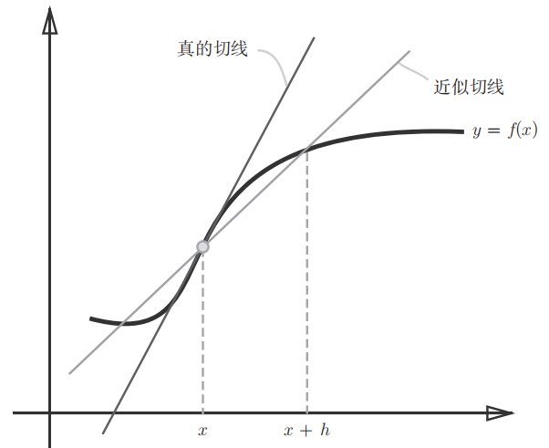
用中心差分的方法可以一定程度上减小误差。也就是计算函数 f 在 (x + h) 和 (x − h) 之间的差分。（(x + h) 和 x 之间的差分也叫前向差分）

# 中心差分
def numerical_diff(f, x):
    h = 1e-4  # 0.0001
    return (f(x + h) - f(x - h)) / (2 * h)

偏导数 ¶

\[ f(x)=x_0^2+x_1^2 \]

def function_2(x):
    return x[0]**2 + x[1]**2

求 x0 = 3, x1 = 4 时，两个偏导数

def function_2(x):
    return x[0]**2 + x[1]**2


def function_tmp1(x0):
    return x0*x0 + 4.0**2.0


def function_tmp2(x1):
    return 3.0**2.0 + x1*x1


numerical_diff(function_tmp1, 3.0) #6.00000000000378
numerical_diff(function_tmp2, 4.0) #7.999999999999119

梯度 ¶

import numpy as np
import matplotlib.pylab as plt
from mpl_toolkits.mplot3d import Axes3D


def _numerical_gradient_no_batch(f, x):
    h = 1e-4 # 0.0001
    grad = np.zeros_like(x)
    
    for idx in range(x.size):
        tmp_val = x[idx]
        x[idx] = float(tmp_val) + h
        fxh1 = f(x) # f(x+h)
        
        x[idx] = tmp_val - h 
        fxh2 = f(x) # f(x-h)

        grad[idx] = (fxh1 - fxh2) / (2*h)
        x[idx] = tmp_val # 还原值
        
    return grad

def function_2(x):
    return x[0]**2 + x[1]**2

if __name__ == '__main__':
    grad = _numerical_gradient_no_batch(function_2, x=np.array([3.0, 4.0]) )
    print(grad)

梯度法 ¶

损失函数很复杂，参数空间很庞大，无法想象形态，不知道哪里是最小值，所以需要利用梯度寻找最小值（或尽可能小的值），这就是梯度法。

\[ x_0=x_0-\eta\frac{\partial f}{\partial x_0}\\ x_1=x_1-\eta\frac{\partial f}{\partial x_1} \]

\(\eta\) 表示更新量，神经网络称之为学习率（learning rate），学习率决定在一次学习中，应该学习多少，以及在多大程度上更新参数。

学习率一般会一边改变学习率的值，一边确认学习是否正确进行了

def gradient_descent(f, init_x, lr=0.01, step_num=100):
    x = init_x
    for i in range(step_num):
        grad = _numerical_gradient_no_batch(f, x)
        x -= lr * grad
    return x

像学习率这样的参数称为超参数。这是一种和神经网络的参数（权重和偏置）性质不同的参数。相对于神经网络的权重参数是通过训练数据和学习算法自动获得的，学习率这样的超参数则是人工设定的。一般来说，超参数需要尝试多个值，以便找到一种可以使学习顺利进行的设定。

神经网络的梯度 ¶

把梯度法迁移到神经网络，其实是指损失函数关于权重参数的梯度

\[ W= \left( \begin{array}{l} w_{11} & w_{12} & w_{13}\\ w_{21} & w_{22} & w_{23} \end{array} \right)\\ \frac{\partial L}{\partial W}= \left( \begin{array}{l} \frac{\partial L}{\partial w_{11}} & \frac{\partial L}{\partial w_{12}} & \frac{\partial L}{\partial w_{13}}\\ \frac{\partial L}{\partial w_{21}} & \frac{\partial L}{\partial w_{22}} & \frac{\partial L}{\partial w_{23}} \end{array} \right) \]

以一个简单的神经网络为例，来实现求梯度的代码

import numpy as np
import os
import sys
sys.path.append(os.pardir)
from common.functions import softmax, cross_entropy_error
from common.gradient import numerical_gradient

class simpleNet:
    def __init__(self):
        self.W = np.random.randn(2, 3) #用高斯分布进行初始化
    
    def predict(self, x):
        return np.dot(x, self.W)
    
    def loss(self, x, t):
        z = self.predict(x)
        y = softmax(z)
        loss = cross_entropy_error(y, t)
        return loss

net = simplenet()
print(net.W) #权重参数

x = np.arrary([0.6,0.9])
p = predict(x)
print(p) #预测值

np.argmax(p) # 最大值的索引

t = np.array([0, 0, 1]) # 正确解标签
net.loss(x, t)

def f(W):
    return net.loss(x, t)

dW = numerical_gradient(f, net.W)
print(dW)

学习算法的实现 ¶

前提神经网络存在合适的权重和偏置，调整权重和偏置以便拟合训练数据的过程称为“学习”。神经网络的学习分成下面4个步骤。

步骤 1（mini-batch） 从训练数据中随机选出一部分数据，这部分数据称为mini-batch。我们的目标是减小mini-batch的损失函数的值。

步骤 2（计算梯度） 为了减小mini-batch的损失函数的值，需要求出各个权重参数的梯度。梯度表示损失函数的值减小最多的方向。

步骤 3（更新参数） 将权重参数沿梯度方向进行微小更新。

步骤 4（重复） 重复步骤1、步骤2、步骤3。

神经网络的学习按照上面 4 个步骤进行。这个方法通过梯度下降法更新参数，不过因为这里使用的数据是随机选择的 mini batch 数据，所以又称为随机梯度下降法 (SGD)

import sys
import os
import numpy as np
# fmt:off
sys.path.append(os.pardir)
from common.functions import *
from common.gradient import numerical_gradient
# fmt:on


class TwoLayerNet:
    # 初始化权重
    def __init__(self, input_size, hidden_size, output_size, weight_init_std=0.01):
        self.params = {}
        self.params['W1'] = weight_init_std * \
            np.random.randn(input_size, hidden_size)
        self.params['b1'] = np.zeros(hidden_size)
        self.params['W2'] = weight_init_std * \
            np.random.randn(hidden_size, output_size)
        self.params['b2'] = np.zeros(output_size)

    def predict(self, x):
        W1, W2 = self.params['W1'], self.params['W2']
        b1, b2 = self.params['b1'], self.params['b2']

        a1 = np.dot(x, W1) + b1
        z1 = sigmoid(a1)
        a2 = np.dot(z1, W2) + b2
        y = softmax(a2)
        return y

    def loss(self, x, t):
        y = self.predict(x)
        return cross_entropy_error(y, t)

    def accuracy(self, x, t):
        y = self.predict(x)
        y = np.argmax(y, axis=1)
        t = np.argmax(t, axis=1)

        accuracy = np.sum(y == t) / float(x.shape[0])
        return accuracy

    def numerical_gradient(self, x, t):
        def loss_W(W): return self.loss(x, t)

        grads = {}
        grads['W1'] = numerical_gradient(loss_W, self.params['W1'])
        grads['b1'] = numerical_gradient(loss_W, self.params['b1'])
        grads['W2'] = numerical_gradient(loss_W, self.params['W2'])
        grads['b2'] = numerical_gradient(loss_W, self.params['b2'])

        return grads

将这个 2 层神经网络实现为一个名为 TwoLayerNet 的类，下面是一个实例

net = TwoLayerNet(input_size=784, hidden_size=100, output_size=10)
print(net.params['W1'].shape)  # (784, 100)
print(net.params['b1'].shape)  # (100,)
print(net.params['W2'].shape)  # (100, 10)
print(net.params['b2'].shape)  # (10,)

x = np.random.rand(100, 784)  # 伪输入数据（100个）
t = np.random.rand(100, 10)   # 伪正确解标签（100笔）

grads = net.numerical_gradient(x, t)  # 计算梯度
print(grads['W1'].shape)  # (784, 100)
print(grads['b1'].shape)  # (100,)
print(grads['W2'].shape)  # (100, 10)
print(grads['b2'].shape)  # (10,)

权重使用符合高斯分布的随机数进行初始化，偏置使用 0 进行初始化。。predict 计算到隐藏层的结果。loss 计算输出和结果的交叉熵误差，accuracy 则计算准确度。numerical_gradient 计算参数的梯度。

mini-batch 的实现 ¶

# coding: utf-8
import sys, os
sys.path.append(os.pardir)  # 为了导入父目录的文件而进行的设定
import numpy as np
import matplotlib.pyplot as plt
from dataset.mnist import load_mnist
from two_layer_net import TwoLayerNet

# 读入数据
(x_train, t_train), (x_test, t_test) = load_mnist(normalize=True, one_hot_label=True)

network = TwoLayerNet(input_size=784, hidden_size=50, output_size=10)

iters_num = 10000  # 适当设定循环的次数
train_size = x_train.shape[0]
batch_size = 100
learning_rate = 0.1

train_loss_list = []
train_acc_list = []
test_acc_list = []

iter_per_epoch = max(train_size / batch_size, 1)

for i in range(iters_num):
    batch_mask = np.random.choice(train_size, batch_size)
    x_batch = x_train[batch_mask]
    t_batch = t_train[batch_mask]
    
    # 计算梯度
    #grad = network.numerical_gradient(x_batch, t_batch)
    grad = network.gradient(x_batch, t_batch)
    
    # 更新参数
    for key in ('W1', 'b1', 'W2', 'b2'):
        network.params[key] -= learning_rate * grad[key]
    
    loss = network.loss(x_batch, t_batch)
    train_loss_list.append(loss)
    
    if i % iter_per_epoch == 0:
        train_acc = network.accuracy(x_train, t_train)
        test_acc = network.accuracy(x_test, t_test)
        train_acc_list.append(train_acc)
        test_acc_list.append(test_acc)
        print("train acc, test acc | " + str(train_acc) + ", " + str(test_acc))

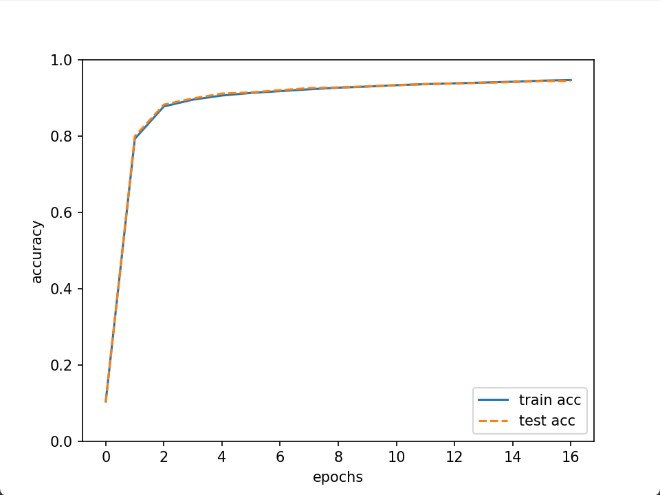
# 绘制图形
markers = {'train': 'o', 'test': 's'}
x = np.arange(len(train_acc_list))
plt.plot(x, train_acc_list, label='train acc')
plt.plot(x, test_acc_list, label='test acc', linestyle='--')
plt.xlabel("epochs")
plt.ylabel("accuracy")
plt.ylim(0, 1.0)
plt.legend(loc='lower right')
plt.show()