误差反向传播 
约 1106 个字 110 行代码 预计阅读时间 6 分钟
高效计算权重参数的梯度的方法——误差反向传播
链式法则 
传递这个局部导数的原理,是基于链式法则(chain rule)的
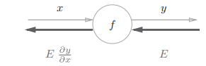
局部导数 \(\frac{\partial y}{\partial x}\) 乘以上游传来的值 \(E\),然后传递给前面的节点。这就是反向传播的计算顺序。实现的原理是链式法则
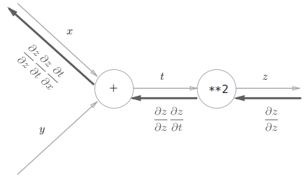
\(z=(x+y)^2\)
可以写成两个式子,反向传播图如下所示 $$ z=t^2\ t=x+y $$
反向传播 
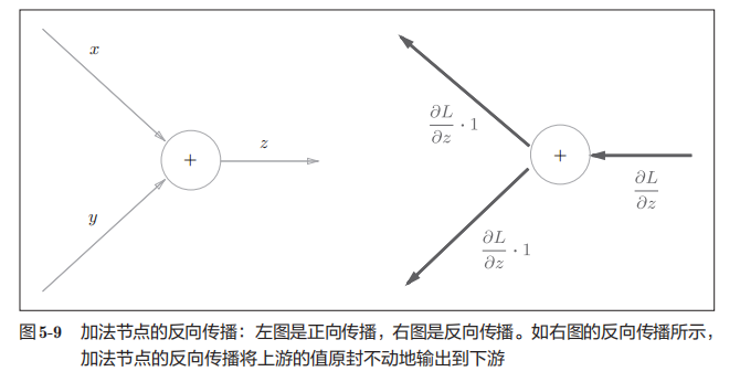
加法节点的反向传播 
加法节点的反向传播将上游的值原封不动地输出到下游
乘法节点的反向传播 
乘法的反向传播会将上游的值乘以正向传播时的输入信号的“翻转值”后传递给下游。翻转值表示一种翻转关系,如图 5-12 所示,正向传播时信号是 x 的话,反向传播时则是 y;正向传播时信号是 y 的话,反向传播时则是 x。
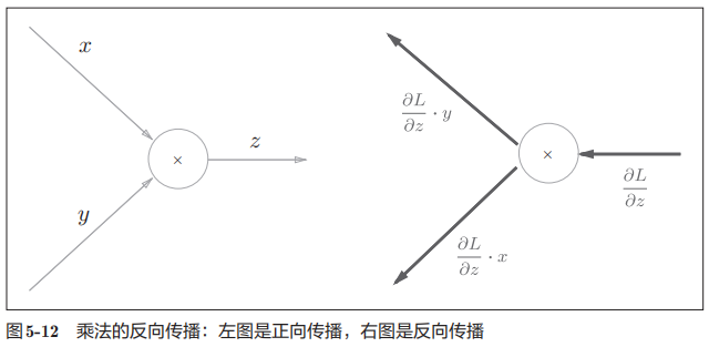
加法的反向传播只是将上游的值传给下游,并不需要正向传播的输入信号。但是,乘法的反向传播需要正向传播时的输入信号值
简单层的实现 
### 乘法层的实现
class MulLayer:
    def __init__(self):
        self.x = None
        self.y = None

    def forward(self, x, y):
        self.x = x
        self.y = y
        out = x * y
        return out

    def backward(self, dout):
        dx = dout * self.y
        dy = dout * self.x
        return dx, dy
用前面苹果的例子
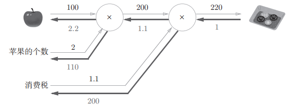
# 买苹果
apple = 100
apple_num = 2
tax = 1.1
#layer
mul_apple_layer = MulLayer()
mul_tax_layer = MulLayer()
#forward
apple_price = mul_apple_layer.forward(apple,apple_num)
price = mul_tax_layer.forward(apple_price,tax)

print(price)# 220
加法层的实现 
class AddLayer:
    def __init__(self):
        pass

    def forward(self, x, y):
        out = x+y
        return out

    def backward(self, dout):
        dx = dout * 1
        dy = dout * 1
        return dx, dy
激活函数层的实现 
ReLU 层 
激活函数 ReLU(Rectified Linear Unit)
可求得导数
也就是说,如果正向传播输入 x 大于 0,那么反向传播时原封不动传递给上游。如果 x 小于 0,那反向传播到此为止。
# ReLU层
class ReLu:
    def __init__(self):
        self.mask = None

    def forward(self, x):
        self.mask = (x <= 0)
        out = x.copy()
        out[self.mask] = 0
        return out

    def backward(self, dout):
        dout[self.mask] = 0
        dx = dout
        return dx
Relu 类有实例变量 mask。这个变量 mask 是由 True/False 构成的 NumPy 数组,它会把正向传播时的输入 x 的元素中小于等于 0 的地方保存为 True,其他地方(大于 0 的元素)保存为 False。
Sigmoid 层 
最终反向传播的输出是 \(\frac{\partial L}{\partial y}y^2\exp{(-x)}\),这个反向传播的值与正向传播的输入 x 和输出 y 相关。简化这个 sigmoid 层表示为
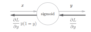
class Sigmoid:
    def __init__(self):
        self.out = None

    def forward(self, x):
        out = 1 / (1 + np.exp(-x))
        self.out = out
        return out

    def backward(self, dout):
        dx = dout * (1.0 - self.out) * self.out
        return dx
Affine/Softmax 层的实现 
Affine 层 
神经网络的正向传播中进行的矩阵的乘积运算在几何学领域被称为“仿射变换”A。因此,这里将进行仿射变换的处理实现为“Affine 层”。
几何中,仿射变换包括一次线性变换和一次平移,分别对应神经网络的加权和运算与加偏置运算。
回顾一下神经网络的正向传播,是一个加权信号的总和,用到了矩阵的乘法
X = np.random.rand(2) # 输入
W = np.random.rand(2,3) # 权重
B = np.random.rand(3) # 偏置

X.shape # (2,)
W.shape # (2, 3)
B.shape # (3,)

Y = np.dot(X, W) + B
(2,) 是一个 1×2 的哦,但是 (2,3) 是 2×3 的矩阵
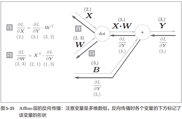
注意,矩阵翻转的同时还要注意转置
批版本的 Affine
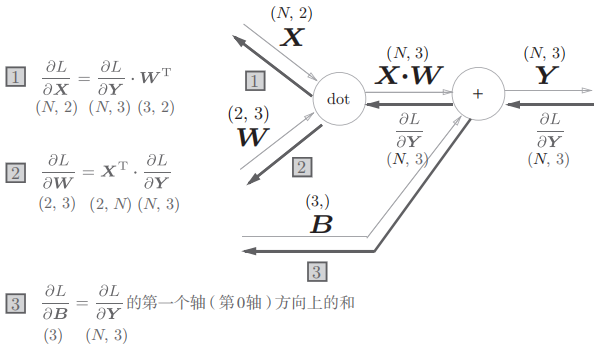
这里还有一个细节,正向传播的时候,虽然偏置看上去是一行的,但是实际加到加权和还是根据输入的行数来的,所以偏置实际上是 N 行的。所以反向传播的时候,传回去还得重新压缩回一行。那就得按列求总和。
#正向传播
>>> X_dot_W = np.array([[0, 0, 0], [10, 10, 10]])
>>> B = np.array([1, 2, 3])
>>>
>>> X_dot_W
array([[ 0, 0, 0],
[ 10, 10, 10]])
>>> X_dot_W + B
array([[ 1, 2, 3],
[11, 12, 13]])
#反向传播
>>> dY = np.array([[1, 2, 3,], [4, 5, 6]])
>>> dY
array([[1, 2, 3],
[4, 5, 6]])
>>>
>>> dB = np.sum(dY, axis=0)
>>> dB
array([5, 7, 9])
Softmax-with-Loss 层 
最后介绍一下输出层的 softmax 函数。前面我们提到过,softmax 函数会将输入值正规化之后再输出
手写数字识别
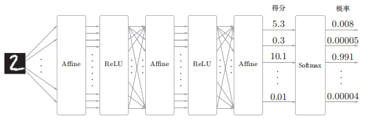
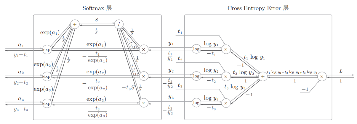
考虑到这里也包含作为损失函数的交叉熵误 差(cross entropy error),所以称为“Softmax-with-Loss层”,内部结构如下
上面的结构有点复杂,下面是简化后的结果
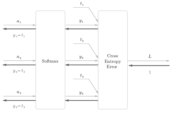
Softmax 层的反向传播得到了(y1 − t1, y2 − t2, y3 − t3)这样“漂亮”的结果。由于(y1, y2, y3)是 Softmax 层的输出
回归问题中输出层使用恒等函数,损失函数使用平方和误差 , 反向传播才是上面这样漂亮的结果
class SoftmaxWithLoss:
    def __init__(self):
        self.loss = None
        self.y = None
        self.t = None

    def forward(self, x, t):
        self.t = t
        self.y = softmax(x)
        self.loss = cross_entropy_error(self.y, self.t)
        return self.loss

    def backward(self, dout=1):
        batch_size = self.t.shape[0]
        dx = (self.y - self.t) / batch_size
        return dx